In my previous post about Piecewise Aggregate Approximation (PAA) I discussed about the algorithm. One of the extensions of PAA leads to Symbolic Aggregate Approximation (SAX). In literature, SAX falls under a group of representation systems which are data-adaptive for time-series and are symbolic. As the name suggests, the algorithm takes a time series and represents it in terms of symbols that are approximate representations of the original time series.

SAX takes a time series of arbitrary length, \(n\), and reduces it to a string of arbitrary length, \(w\). The length of the string is \(w < n\) and typically it is such that \(w \ll n\). The process of SAX first requires that the string is first transformed using the PAA representation which is then symbolised by SAX to form a symbolic representation.

Discretisation

The idea behind the SAX transformation involves discretisation of the time series of length \(n\) to form sequences. The first part of the discretisation is handled by the PAA transformation. The next part of the process is to assign symbols for the sections. One requirement for the second part of this discretisation technique is that the symbols are assigned by equiprobability, the property for a collection of events having the same probability of occurring. This is an easy requirement to fulfill as the normalised time series data have a Gaussian distribution. Therefore for discretisation, the equal sized areas under the Gaussian curve can be used for creating breakpoints in the normalised data for assigning the symbols [1].

1 Breakpoints are a sorted list of numbers \(\beta = \beta_{1}, …, \beta_{a-1}\) such that the area under the Gaussian curve \(\beta_i\) to \(\beta_{i+1} = 1/a\).

These breakpoints can be obtained by looking up a statistical table and can be used to discretise the time series where the coefficients below the smallest breakpoint are mapped to the letter \(a\) while the coefficients greater than or equal to the smallest breakpoint and less than the second breakpoint are assigned to the letter \(b\) and so on. A sequence of such symbols is called a word for example bcdfa. A sample code from python to look up the breakpoints for an arbitrary amount of regions from a normal distribution function is below.

# Python
import numpy as np
import scipy as sp

def lookupEquiprobableRegions(word_length):
    """Look up equiprobable regions from a normal distribution"""
    regions = np.arange(0, word_length, 1) / word_length
    return sp.stats.norm.ppf(regions)

The above function uses the Percent Point Function (PPF) which is the inverse of the cumulative distribution function and is also called the inverse distribution function (for example, in Matlab it is a function called norminv) [2]. The principle being that for a given distribution function, the probability that the given variable is less than or equal to \(x\) for a given \(x\) is computed. In the python example, the breakpoints are defined by the regions variable which takes the word_length and creates an array of the positions of the breakpoints on the normal distribution. The final returned output are the breakpoint values.

2 Word is a subsequence \(C\) of a length \(n\) that can be represented as a word. If \(\alpha_i\) is the i-th element of the alphabet, then mapping the approximation of PAA to a word \(\hat{C}\) is obtained using \(\hat{C} = \alpha_j\) if \(\beta_{j-1} \leq \bar{C_i} \lt \beta_j\). This defines the symbolic representation of the series.

With the above lookup table ready, the time series data can now be converted to the symbolic representation. The method of doing this is to map the different elements of a string section, in this case, the ascii alphabet sequence to the breakpoint regions. The example for this study is the same 7-point PAA graph from the previous blog post. The only difference being that the graph is now normalised. As explained above, the symbol is chosen such that the PAA sequence \(\bar{C_i}\) is greater than equal to the breakpoint \(\beta_{j-1}\) or less than the breakpoint \(\beta_j\).

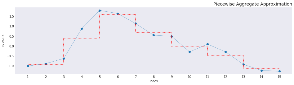
The seven breakpoint regions for the graph are straightforward to gather from the lookup function. The corresponding symbols to choose from are the first 7 alphabets, abcdefg. The code to assign the symbols is given below:

sax = list()
regions = np.array(tuple(zip(eqprob, eqprob[1:])))
# -- loop through the array
for val in paa_arr:
    high_bound = np.where(test[:, 1] >= val)[0]
    low_bound = np.where(test[:, 0] <= val)[0]
    try:
        intersect = np.intersect1d(
            bound_high, bound_low)[0]
    except IndexError as e:
        intersect = bound_low.max() + 1
    if val < 0:
        intersect += 1
    sax.append(intersect)
# -- print the symbolic representation
print("Symbolic Representation is: %s" % (''.join(sax)))

For the above graph, the symbolic representation of the line is cegfedb. The assignment operation is undertaken in such a way that for the negative values, it is the highest bin plus 1 that is lesser than the number and for the positive values, it is the lowest bin minus 1 that is greater than the number. This makes sure that the values are between the values that bound that particular number. And the word is assigned in two parts, one for the higher bound values and then the lower bound values. One thing for the reader to note is that this code is not vectorised and therefore would be quite slow for large time series sequences.

How is SAX useful?

A few application domains of SAX are in clustering, querying by content and indexing, detection of anomalous / novel behavior in the dataset, and visualisation using text-trees. The aspect of the visualisation of trees is quite interesting as different time-series sections could have different word compositions. However, since the text is a reliable pattern, a tree-like structure can be built using the symbol position. For example, all data groups starting with a can be taken and checked if the following symbolic patterns are repetitive or whether there is anomalous behavior as seen by for example an outlying value.

Footnotes (and) References

Note: I have skipped out on one of the important parts of the article discussing the distance measure for the time series. That is, the ability to compare the similarity of two time series arrays of the same length \(n\). It is important that the new representation proposed lower-bounds a distance measure and in the article, the authors go in great detail on the proof that SAX lower-bounds the Euclidean distance measure. You can find the proof from the article linked at the references section below.

[1] Jessica Lin, Eamonn Keogh, Li Wei, Stefano Lonardi, - Experiencing SAX: A novel symbolic representation of time series

[2] Percent Point Function - ITL NIST - visited on 2018-06-26

[3] SeninP/saxpy - Github Rep