I’ve been working with time series datasets quite a lot lately. One of the common requirements in time series datasets is to find clusters or common trends across different periods during a day or a week. However, these are pretty complex operations over time if the dimensionality of certain trends are longer than a day or a week. One of the algorithms that is designed to reduce the dimensionality is called Piecewise Aggregate Approximation (from now on, PAA).
Background
Commonly, time series datasets and databases tend to grow to extremely large sizes. Sampling consistently is a requirement in a lot of cases where these databases are involved. During this process, the ability to search through the database becomes unreasonably time consuming. One algorithm that assists in performing these searches quickly and efficiently is the PAA discussed in a paper by Keogh et al.[1] from 2001. The basic idea behind the algorithm is: to reduce the dimensionality of the input time series by splitting them into equal-sized segments which are computed by averaging the values in these segments. The benefits of doing this will be explained at the end of this post and in the following posts.
Dimensionality Reduction
Assuming a time series \(Y = Y_1, Y_2, …, Y_n\) of length (n) to be split or reduced into a series \(X = X_1, X_2, …, X_m\) where \(m \leq n\), the overall equation describing the elements in the reduced series can be summed up by the formula:
$$\bar{X}_i = \frac{m}{n} \cdot \sum_{j=n/N(i-1) + 1}^{(n/M)\cdot i} x_j$$
The above equation provides the mean of the elements in the equi-sized frame which makes up the vector of the reduced dimensional series. There are immediate special cases however,
- \(m = n\): The reduced series is exact copy of the original sequence.
- \(m = 1\): The reduced series is the mean of the original sequence.
The second case is a special case where the result is a piecewise constant approximation. This is the root for the name piecewise aggregate approximate as other cases involve the mean of values within a frame. That is that the original input vector is split into frames and the mean of the values in the frame are computed. The most interesting aspect of the algorithm is how it creates these equi-sized frames. It is important to note here that before the actual mean approximates of the windows are computed, the input vector is Z-normed. Z-normalization is the process of normalizing the data to zero mean and zero unit of energy which is to say that the mean is 0 and the standard deviation is approximately 1. Once that is performed, the piecewise approximates can be computed. However there are two cases to consider. The Python code for the case when ((m \leq \n\) and \(m \bmod n == 0\) is given as follows:
# Python
Y = np.array  # input vector
paa = int     # number of outputs in the output vector

if Y.shape[0] % paa == 0:
    sectionedArr = np.array_split(Y, paa)
    res = np.array([item.mean() for item in sectionedArr])
When the remainder is zero, we can essentially split the input vector into equal sizes easily. And the mean can be calculated for these equal sized frames. The same equation is not applicable for the case when \(m \lt n\) and \(m \bmod n \gt 0\). When the remainder is greater than zero, the frames can no longer be equi-sized easily. There is an imbalance to how the frames can be built. It is now required that the frame be resized so that the each element of the output series is the mean of an equi-sized frame of the input vector. An example code looks like this:
# Python
import numpy as np

Y = np.array  # input vector
paa = int     # number of outputs in the output vector

if Y.shape[0] % paa != 0:
    valuespace= np.arange(0, Y.shape[0] * paa)
    output_index = value_space // Y.shape[0]
    input_index = value_space // paa
    uniques, nUniques = np.unique(output_index, return_counts=True)
    res = [input[indices].sum() / input.shape[0] for indices in
           np.split(input_index, nUniques.cumsum())[:-1]]
The above code is a modified version of the original version in R-lang\(^{a}\). The first step is to create the overall space by multiplying the size of the input array \(Y\) with the size of required output frame, \(X\), i.e., \n \cdot m\) where \(n\) and \(m\) are the lengths of the input and output vectors respectively. Assuming an input vector \(Y\) of length 15 and the size of the output vector \(X\) is to be 7, the total exploded space has 104 elements. With this as a foundation, we can divide the vector by the length input vector and the length of the output vector to get two index vectors.
# Output Index
array([0, 0, 0, 0, 0, 0, 0, 0, 0, 0, 0, 0, 0, 0, 0,
       1, 1, 1, 1, 1, 1, 1, 1, 1, 1, 1, 1, 1, 1, 1,
       2, 2, 2, 2, 2, 2, 2, 2, 2, 2, 2, 2, 2, 2, 2,
       3, 3, 3, 3, 3, 3, 3, 3, 3, 3, 3, 3, 3, 3, 3,
       4, 4, 4, 4, 4, 4, 4, 4, 4, 4, 4, 4, 4, 4, 4,
       5, 5, 5, 5, 5, 5, 5, 5, 5, 5, 5, 5, 5, 5, 5,
       6, 6, 6, 6, 6, 6, 6, 6, 6, 6, 6, 6, 6, 6, 6])
Taking the total of 104 elements, the division by the input vector size and the output array size creates the two index vectors. The one above, called the output_index, creates the number of elements in the input index vector that make up one single frame for the index in the output vector equal to the unique values. The array below named the input_index, provides the indices of the input vector \(Y\) that should be summed up from the dataset.
# Input Index
array([ 0,  0,  0,  0,  0,  0,  0,  1,  1,  1,  1,  1,  1,  1,  2,
        2,  2,  2,  2,  2,  2,  3,  3,  3,  3,  3,  3,  3,  4,  4,
        4,  4,  4,  4,  4,  5,  5,  5,  5,  5,  5,  5,  6,  6,  6,
        6,  6,  6,  6,  7,  7,  7,  7,  7,  7,  7,  8,  8,  8,  8,
        8,  8,  8,  9,  9,  9,  9,  9,  9,  9,  10, 10, 10, 10, 10,
        10, 10, 11, 11, 11, 11, 11, 11, 11, 12, 12, 12, 12, 12, 12,
        12, 13, 13, 13, 13, 13, 13, 13, 14, 14, 14, 14, 14, 14, 14])
Let me explain it further, the two index vectors are of the same size. If we take the unique elements in the output_index, we arrive at 15 repetitions of the numbers [0, 1, 2, 3, 4, 5, 6]. Since Python uses 0 based indexing, the values start from 0. This is infact the index markers for the output vector \(X\) which we assumed to be of length 7. Each unique number is repeated 15 times. In other words, that 15 element repetition represents the window which computes the mean of that position in the output vector \(X\). The value filling the \(\bar{X}_i\) are the elements from the input vector \(Y\) represented by the 15 positions for each of the output index. So the elements can be given by \(^{b}\):
$$ X_i = \frac{\sum_{j=z}^{z+n} Y_{i}}{n}, J \in I_{in} $$
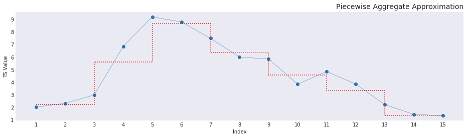
Where \(n\) is the number of elements in the input vector \(Y\) and \(I_{in}\) is the input index with \(z\) equalling the cumulative sum vector of the nunique values of the input index. The basis of doing that creates the graph as shown below. Additionally, \(j\) increases as a cumulative sum of the repetitions of unique values in the output_index. As in the first interval is \([0, n]\), and the second interval is \([n, 2n]\) and so on. This makes sure that the window sizes increase as the overall size of the elements increase. In our example the element \(X_0\) will be filled by the mean of the values indexed in \(Y\) by the first 15 elements in the input_index. The second element \(X_1\) would be mean of the values in \(Y\) provided by each of the indices from the 15th element to the 30th element and so on. This method of summation makes sure that elements added to the right of the sliding window actually influences the frame. This influence can be seen in the input index code. Without a sliding window, the elements are split unevenly and the values entering on the right aren’t influencing the frame in any discernible way thereby changing the value that that approximates the frame in question. The reduced dimensionality after PAA gives a step graph, as seen below, that shows the reduced dimensionally while preserving information about the original data and simplifying the shape in a way that comparisons are possible as a euclidean distance (more on this on a later post).
What does this help with?
PAA leads directly to another representation called Symbolic Aggregate approXimation, shortened to SAX. This takes the reduced dimensionality and assigns a string representation to the graph. By providing a string representation, the overall data that is required to be stored less than other data mining methods such as Discrete Fourier Transform (DFT) and Wavelet Transformation. My exposure comes from trying to compare and cluster for example, power consumption data sampled every 15 minutes. By breaking the profiles into daily cycles and approximating it provides a quick overview on how many different profiles exist within the data collected i.e., speeds up the process of similarity searches and comparison against other profiles using euclidean distance measures. In future posts, I’ll talk a bit more in detail about how this algorithm helps in comparing profiles easily and effectively. Later on, I’ll delve in a bit more into the string approximation of the SAX algorithm.
You can find the code to the graphs and the general PAA code from my jupyter-notebooks repo vignkri/Notebooks. You can leave me comments by contacting me through my github.
Footnotes (and) References
a) This code is a numpy driven trial rather than building it like most other answers using while or for-loops. In pandas using daily profiles, this becomes far easier as DataFrame.resample('freq').mean() can be used to do the same. As 24H profiles are quite easy to break down into 3H, 4H, 6H, 8H approximates. The original code which was rebuilt can be found at: JMotif/jmotif-R
[1] Eamonn Keogh, Kaushik Chakrabarti, Michael Pazzani, and Sharad Mehrotra. Dimensionality reduction for fast similarity search in large time series databases. Knowledge and information Systems, 3(3), 263-286, 2001.